iTTT (WIP)

08 Apr, 2026

TLDR

• A sequence modelling architecture in a new memory class: O(1) memory at training time.
• Works as a training-free drop-in for existing LLMs, and improves with finetuning.
• Outperforms dense attention when training from scratch at 32K context length (1B params, 4B tokens).
• Gracefully extrapolates beyond the training sequence length.

Links

Code: aklein4/iTTT @ github

Introduction

I believe that the solution to extreme-context sequence modelling and continual learning will have the following properties:

1. Convergence and Extrapolation Guarantees: Existing long-context architectures cannot reliably extrapolate beyond their training length; once their training sequence length is exceeded they either catastrophically fail or act like a sliding context window. Contrast this with gradient descent, where models keep getting better at predicting future data no matter how much it has already seen ¹. The difference is that gradient descent is convergent, which is to say that you end up with defined behavior (interpolating the training data) if you run it infinitely. A true infinite-context or continual learning solution should do the same.

2. O(1) Training Memory and O(N) Training Compute: Sub-quadratic sequence modelling architectures, like SSMs and Linear Attention are often advertised as using O(1) memory and O(N) compute. However, that only applies at inference time. At training time, they use O(N) memory (for storing activations at every position). Activation checkpointing can bring memory down to O(log N) memory at the cost of O(N log N) compute. I believe that for practically scaling to truly massive training context lengths, the standard should be O(1) memory and O(N) compute at training time.

3. Serial Circuit Complexity: The Serial Scaling Hypothesis lays this concept out thoroughly. In short, parallelizable architectures like transformers and SSMs can only solve problems with TC^0 complexity. Many problems including cellular automata, many-body mechanics, and math QA are inherently serial; they cannot be natively solved with TC^0 architectures. Chain-of-thought reasoning provides a work-around to this problem, but has practical limitations. To reason at the level of humans (whose brains probably operate in serial), architectures should exhibit serial complexity. However, this comes at the cost of unparallelizable training and inference.

I also believe that viral and impactful research has the following properties:

1. Simplicity and Ease-of-Implementation: The average researcher, engineer, or hobbyist should be able to read your research paper, understand it, and implement it without specialized knowledge. I believe that this is why test-time training architectures like Titans have not caught on yet; they require custom kernels and low-level code optimization to run with practical speed and memory. Therefore, new ideas should strive to be implementable using only python-level code.

2. Compatibility with Existing Libraries: Attention and transformers have deeply embedded themselves at the core of the ML software stack. To break through, a radical new architecture would need to be significantly better; slightly better is not enough to overcome the technical debt. Therefore, any new architectures should be as compatible with existing implementations as possible.

Methods

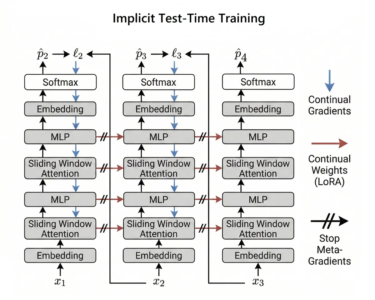
iTTT (Implicit Test-Time Training) is a new sequence-modelling architecture that has been designed to fit all of the design criteria listed above. It operates similar to recent methods like End-to-End Test-Time Training. However, iTTT does not backpropagate through time, instead relying on implicit alignment between continually updated states and fixed parameters.

At the implementation level, iTTT performs continual learning on overlapping chunks of context. At each step, the model takes in the current chunk and the previous chunk. Local interactions are modelled using attention to perform next-token prediction on the current chunk. The "continual gradients" of the resulting loss are then backpropagated through the model into dynamic "continual weights".

How this fulfills the design criteria above:

1. Convergence and Extrapolation Guarantees: The model converges to a known distribution, which is the distribution of overlapping chunks discounted (not necessarily predictably) by how recent they are. It doesn't matter what the frozen weights are; as long as the gradients of the continual state are pre-conditioned in a valid way and the continual learning rate is not too large, the continual weights will converge. The fact that the continual state is constrained to LoRAs also serves to minimize the divergence between the continually learned distribution and the base distribution, which we speculate could induce bayesian-like inference. There are also some clever ways that convergent in-context reinforcement learning could be induced, which we will add here in the future.
2. O(1) Training Memory and O(N) Training Compute: Since we don't backpropagate through time, we can discard the activations of previous chunks. As we slide across the context window, this keeps our training memory constant. It is also obvious that the training compute is O(N).
3. Serial Circuit Complexity: We will formalize this in the future. For now, the reader may trace the computation path in the diagram above to see that the depth of the circuit increases with context length.

The key is that iTTT is not the same as just adding LoRAs to a model post-hoc, because we can meta-learn the fixed parameters and optimizer parameters (like learning rate) to best scaffold the continual learning updates. This is not dissimilar to meta-learning algorithms like MAML and Reptile.

Continual Weights

iTTT maintains a set of continual weights which are iteratively updated as the model ingests new context. In the current version of iTTT, these continual weights take the form of LoRA adapters. Formally, given an existing linear module with weight $W\in {ℝ}^{d_{out},d_{in}}$, rank $r$ iTTT adds a down projection matrix $D\in {ℝ}^{r,d_{in}}$ and an up projection matrix $U\in {ℝ}^{d_{out},r}$:

We have found that the most efficient and stable method is to keep U fixed at inference time, and only update the $D$ matrix with continual gradients. This means that given the temporary state $D_{t-1}$, the forward pass to compute the logits of chunk $C_t$ is given by:

Any linear module in the model can be modified to use continual weight LoRAs. At present, we are only adding them to the MLP down_proj, attention Q, and attention O modules. The MLP down_proj module appears to be the most important for iTTT, as its larger $d_{in}$ dimension ² decreases the interference between different query vectors ³ when the continual weights are viewed as linear Fast Weights.

Initialization

When converting pretrained models into the iTTT architecture, it is important to change the existing behavior of the model as little as possible. Therefore, we initialize $D$ with zeros. This means that $UDx=0$, so until the continual weights have been updated the model's outputs are exactly the same as before.

We initialize the up projection $U$ using the top $r$ singular components of $W$. Concretely, if the SVD of $W$ is $A\Sigma V=W$ and $A_r$ and ${\Sigma }_r$ are the vectors and values of the top $r$ singular components, then we initialize $U=A_r{\Sigma }_r$. This PiSSA-like initialization makes the continual weight LoRAs operate in the most impactful subspace of $W$, and also puts the LoRA weights on the same scale as the values of $W$.

Update Rule

In addition to our LoRA down projection $D\in {ℝ}^{r,d_{in}}$, our continual state contains a momentum matrix $M\in {ℝ}^{r,d_{in}}$. Both of $D$ and $M$ are zeroed at the start of a context.

For consecutive chunks $C_{t-1},C_t$ of length $L_C$, let $X\in {ℝ}^{L_C,d_{in}}$ be the activations going into $D$ at a given iTTT layer and $G_c\in {ℝ}^{L_C,r}$ be the continual gradients coming back to $D$ from the continual loss ${\mathcal{L}}_{\mathcal{c}}=-\log p_{\theta }(C_t|C_{t-1})$.

We first update the momentum using an exponential moving average parameterized by $\beta$ (which is a fixed hyperparameter):

We then update the $D$ continual weights using a Scaled Muon gradient step. Here $\lambda$ is the continual learning rate.

This update rule is similar to those used by previous KV-binding TTT algorithms like ATLAS.

Finetuning

In addition to training-free plug-and-play improvement, you can also finetune (or pretrain from scratch) an iTTT model to significantly improve its performance, which is similar to meta-learning around the continual weight updates. This is done by iterating over the chunks in training sequences and applying the update rule above.

Notably, we do not calculate the finetuning gradients of the continual states $D$ or $M$. Instead, we allow them to be naturally shaped by the activations going into linear layers and the greedy gradients coming back. This induces first-order meta-learning dynamics similar to MAML and Reptile. This is also justified by the findings of Direct Feedback Alignment which show that models can adapt to imperfect gradients and states.

Detaching the continual state and not backpropagating through time allows us to discard the activations and states of chunks that we have processed, instead of storing them for later backpropagation. This is the key that gives iTTT true O(1) training memory requirements.

A big advantage that finetuned iTTT models have over plug-and-play ones is that we can finetune the continual learning rate $\lambda$ (first introduced in the update rule above). For plug-and-play models, we use a single fixed learning rate (we have found 1e-3 to work well). In the finetuning regime, we instead train a full matrix of learning rates for every iTTT module $\lambda \in {ℝ}^{r,d_{in}}$. Individual learning rates for each element gives allows the model to adjust how much each input element connect to each output element at continual learning time, and enables "multi-head" behavior ⁴. We parameterize out continual learning rates as follows, where ${\lambda }_0$ is a fixed hyperparameter (again often 1e-3) and ${\lambda }_{learned}$ are learnable parameters:

We emphasize that these learning rates are not changed during continual learning time, only at finetuning time.

Experiments (drop-in)

Setup

We initialize our models using the pretrained HuggingFaceTB/SmolLM2-360M language model. For our data, we use the LongABC dataset from LongAttn which is optimized for long-range interactions. We truncate the data to 32K context lengths and remove shorter examples.

For the runs below, we use an iTTT LoRA rank of 256. During finetuning, all parameters in the model are trained. The chunk size is set to 512 and the momentum $\beta$ is set to $0.75$. Meta learning rates are scaled by a base value of 1e-3. A batch size of 32 sequences (1M tokens) is used for finetuning.

The baseline is represented by a chunk-wise sliding window model that is equivalent to an iTTT model with a meta learning rate of 0.

Results

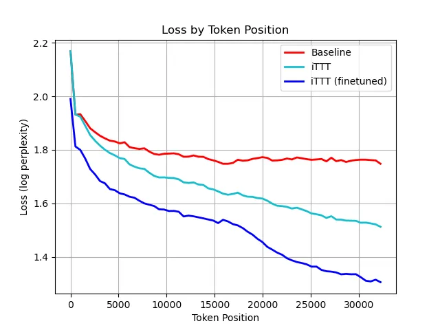
Above, we see the language modelling loss at different token positions for a baseline model, drop-in iTTT (no finetuning), and an iTTT model that has been finetuned for 3K steps (~3B tokens).

iTTT significantly outperforms the baseline, and is further improved through finetuning. It is very important to see that iTTT works without finetuning, because that means it could bring long-context modelling and continual learning to large models with almost zero upfront cost. It also implies that iTTT carries a strong indictive bias towards the behavior we want, which could help it extrapolate to unprecedented context lengths.

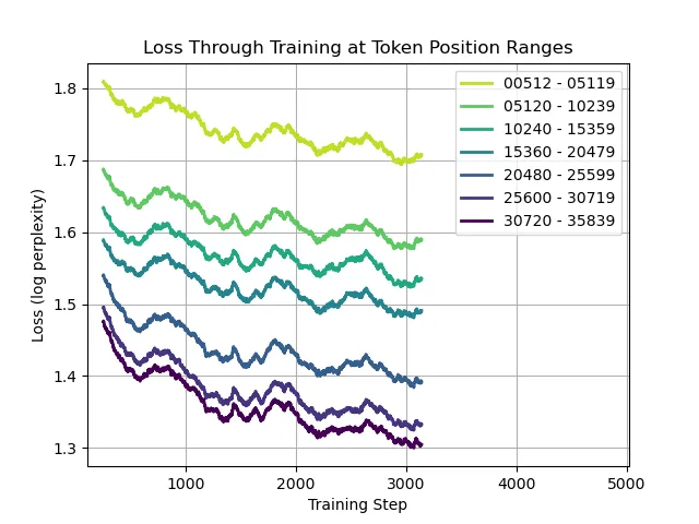
This graph shows how the loss at different token position ranges evolves during finetuning.

We see that the loss in all ranges decreases. Notably, the loss decreases more at later positions (~0.18 $\Delta$) than at early positions (~0.10 $\Delta$). This is evidence that the model is learning to make use of information in the state, even though the state is not directly optimized through backpropagation-through-time.

Experiments (training from scratch)

Setup

We initialize our models from scratch with 1B parameters. Outside of the iTTT mechanisms, the models are standard Llama architectures. We use the SmolLM2 tokenizer. For our data, we use the LongABC dataset from LongAttn which is optimized for long-range interactions. We truncate the data to 32K context lengths and remove shorter examples.

For the iTTT model, we use chunk size 1024, continual LoRA rank 512, continual momentum $\beta =0.9$ (with a slightly modified Muon optimizer for continual updates), base continual learning rate 1e-3, batch size 4M, and learning rate 4e-4.

For the dense attention model, we use RoPE $\theta =5M$, batch size 1M, and learning rate 1.4e-4. We actually expect the smaller batch size to improve training sample efficiency at this scale.

Results

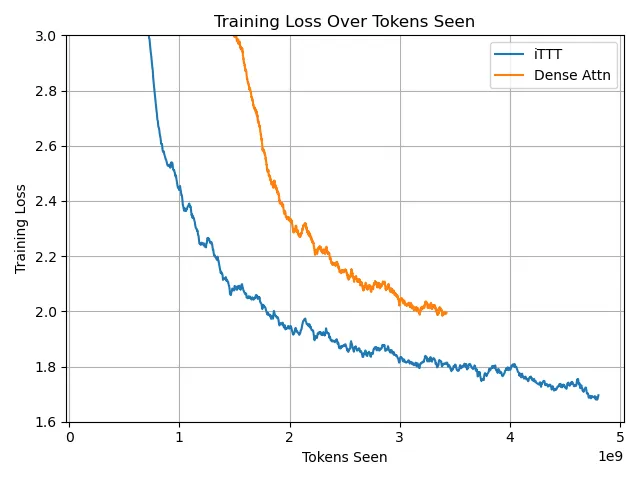
Above, we see the overall cross-entropy loss per token throughout training.

iTTT outperforms the baseline dense attention model at throughout the entire training run. However, we expect the advantage of iTTT to shrink as training continues, as the inductive bias of the architecture becomes less important. In fact, the inductive bias is so strong that iTTT with no training achieves a similar loss (~8.2) to what dense attention reaches after 100M training tokens.

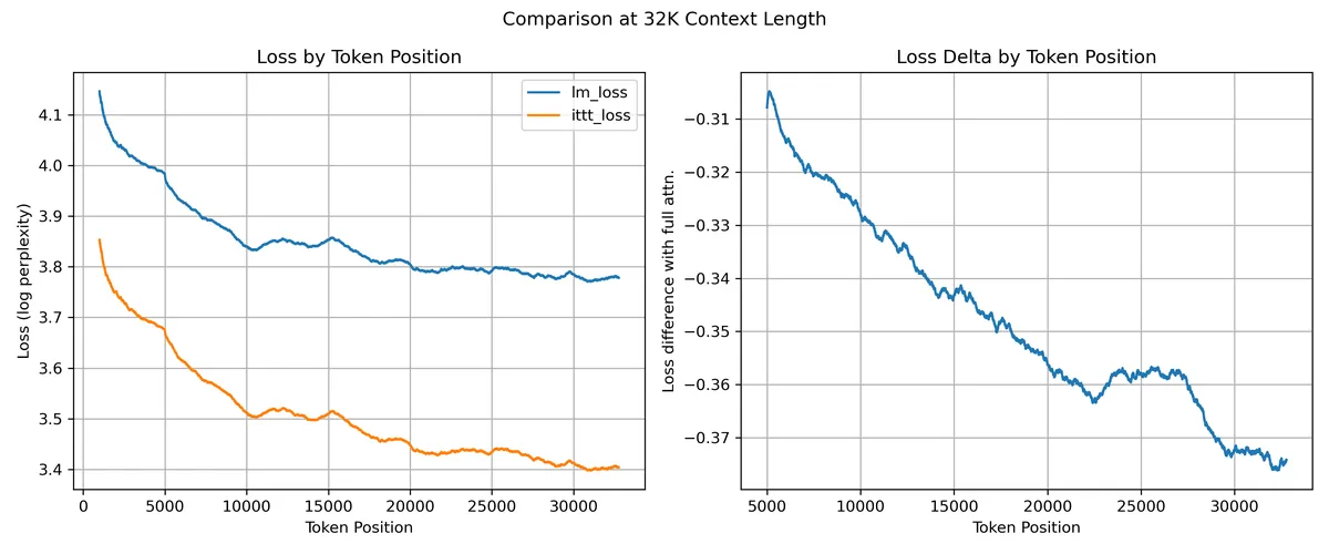
Here we see the loss by token position for the 2B training token checkpoints, as well as the delta between the iTTT and dense attention losses. This loss was measured on the books3 dataset

We see that iTTT outperforms dense attention at all token positions, with the improvement increasing with greater context length.

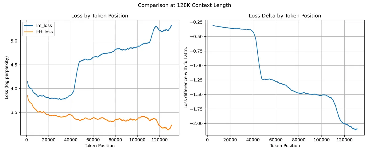
This graph shows the the loss by token position up to 128K for the 2B training token checkpoints, again measured on books3. We again show the delta between iTTT and dense attention. It is important to note that the models were trained with a context length of 32K, so anything beyond that is context length extrapolation.

We see that dense attention (with RoPE position embeddings) catastrophically fails once we move past its training context length. On the other hand, iTTT gracefully extrapolates and continues reducing the perplexity as more context is added. Informally tested up to 1M, are yet to find a context length at which iTTT does not continue decreasing perplexity while extrapolating.

Future Work

iTTT is still a work in progress with much left to do. Among the remaining work is:

1. Scaling to larger models and more training tokens.
2. Thorough evaluations with benchmark suites and needle-in-a-haystack retrieval.
3. Better and more diverse baseline.
4. Convergent in-context reinforcement learning

Footnotes

#project