MonArc

10 Jun, 2024

TLDR

Energy-based models enable native test-time scaling by focusing on each possible output one-at-a-time.
Token-level negative sampling is much more parallelizable than sequence-level sampling.
Token-level EBMs are 2x more data efficient in pretraining than standard autoregressive language models.

Links

Overview

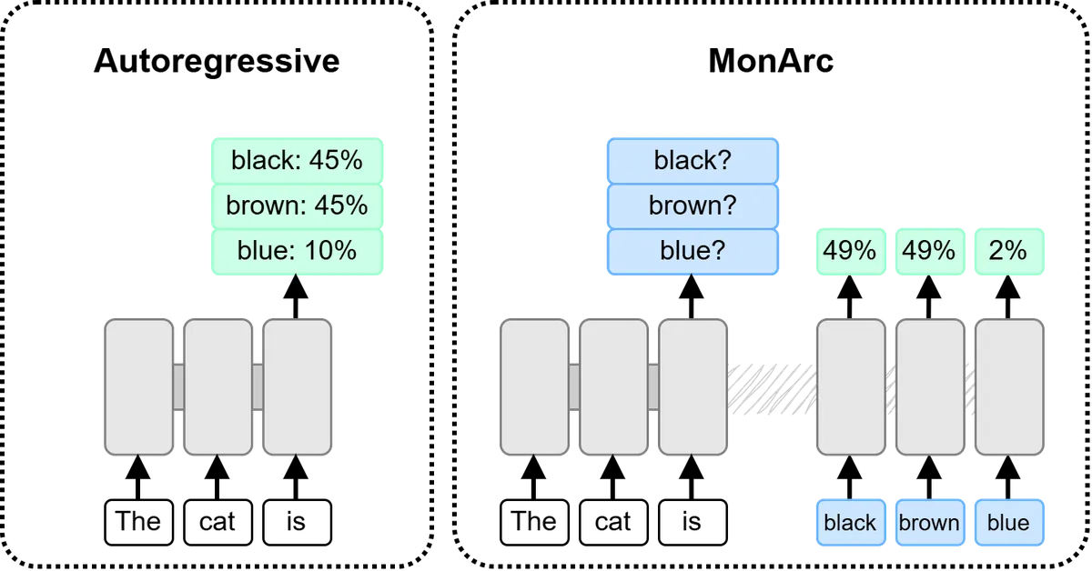
MonArc is a practical method to train energy-based language models (ELMs) using a token-level residual energy framework. In this setup, we have an autoregressive language model (LM) and a residual energy-based model (REBM). At generation time, multiple candidate next-tokens are sampled from the LM. The REBM then processes each candidate individually, and reranks them to decide the final output. This allows the model to 'focus' computation on one candidate at a time.

Compared to previous work that models text using sequence-level REBMs, MonArc is significantly more efficient to train. Residual energy methods typically require 'negative' samples from the base generator distribution in order to discriminate against them. In this case, the base generator distribution is the LM. Sequence-level REBMs require entire sequences to be sampled at training time, which is very slow due to the serial nature of autoregressive sampling. MonArc overcomes this limitation by having the REBM operate on the token level. For MonArc, sampling negatives only requires one parallelizable pass through the LM.

To train our REBM, we introduce a novel loss that we call Regularized Likelihood Maximization (RLM). RLM is similar to Noise Contrastive Estimation (NCE), but is more direct in minimizing the KL-divergence with the target distribution.

When applied with a single causal transformer backbone with separate LM and REBM heads, MonArc shows improved performance over pure LM baselines. This is shown both when training from scratch and when adapting an existing model.

Methods

Formulation

We define our overall model using the standard autoregressive language modelling parameterization.

p_{θ} (x) = \prod_{t = 1}^{T} p_{θ} (x_{t} | x_{< t})

This model is broken into two components. The first component, $p_{L M}$ , is a standard language model that outputs probabilities for each next-token. The second component, $ϕ$ , is an REBM that predicts the residual energy of each possible next-token. This formulation, which includes the (almost) intractable partition function Z, can be seen below.

p_{θ} (x_{t} | x_{< t}) = \frac{p_{L M} (x_{t} | x_{< t}) e^{ϕ (x_{t} | x_{< t})}}{Z (x_{< t})}, Z (x_{< t}) = 𝔼_{x_{t} ~ p_{L M} (x_{t} | x_{< t})} [e^{ϕ (x_{t} | x_{< t})}]

Architecture

We use single causal transformer decoder backbone. The base distribution $p_{L M}$ is calculated the standard way: a softmax function over a vocabulary logits from an output embedding head.

The energy function $ϕ$ is more complicated. Each candidate that we want to calculate the energy for is passed into the transformer individually, and a linear head projects the final hidden state into a scalar energy prediction. We do not separate candidates tokens from those of $x_{< t}$ . Instead, the energy is directly calculated for the most recent token in the sequence. Naively, this means that taking the last energy value from the sequence $x_{< t}$ will yield $ϕ (x_{t - 1} | x_{< t - 1})$ .

Training

During training, $p_{L M}$ is trained using the standard cross-entropy loss. More complicated methods (mostly involving the REINFORCE algorithm) could be used to train $p_{L M}$ more precisely to work with the energy function, but that adds instability and significant complexity. Plus, making $p_{L M}$ as good as possible on its own minimizes the number of candidates that need to be sampled and reranked at inference time.

We first experimented with using the common Noise Contrastive Estimation to train the energy model. This discriminator-like loss can be seen below, where $σ$ is the logistic sigmoid function.

ℒ_{N C E} = 𝔼_{x_{t} ~ p_{d a t a} (x_{t} | x_{< t})} [\log σ (ϕ (x_{t} | x_{< t}))] + 𝔼_{x_{t} ~ p_{L M} (x_{t} | x_{< t})} [\log (1 - σ (ϕ (x_{t} | x_{< t})))]

The thing is, NCE is only empirically correlated with the cross-entropy loss. Its only guarantee is that the optimal solution of $ℒ_{N C E}$ is the ideal energy function, with no guarantees about sub-optimal solutions.

With this in mind, we developed Regularized Likelihood Maximization (RLM), which is more closely linked to the cross-entropy loss. To derive RLM, we start with the cross-entropy in terms of the energy function:

ℒ_{C E} = - 𝔼_{x ~ p_{d a t a} (x)} [\log p_{θ} (x)] = - 𝔼_{x ~ p_{d a t a} (x)} [\log p_{L M} (x) + ϕ (x) - \log Z]

Breaking Z up, we get:

ℒ_{C E} = - 𝔼_{x ~ p_{d a t a} (x)} [\log p_{L M} (x) + ϕ (x) - \log 𝔼_{x ~ p_{L M} (x)} [e^{ϕ (x_{i})}]]

Next, we check the derivative of this function with respect to the energy:

\frac{d ℒ_{C E}}{d ϕ (x)} = - (p_{d a t a} (x) - p_{L M} (x) \frac{e^{ϕ (x)}}{Z})

It is immediately obvious that this won't work, since Z is (almost) intractable. RLM overcomes this using a bold insight: we can just ignore Z in the gradient. This gives us the gradient of the RLM loss:

\frac{d ℒ_{R L M}}{d ϕ (x)} = - (p_{d a t a} (x) - p_{L M} (x) e^{ϕ (x)})

To see why this is a good idea, we work backwards to find the loss that this gradient corresponds with. It turns out that the answer is:

ℒ_{R L M} = ℒ_{C E} + Z - \log Z

This means that the RLM loss is equivalent to the cross-entropy loss plus a $Z - \log Z$ component. This component turns out to be a harmless regularizer that keeps $Z$ close to 1 (and equivalently $\log Z$ close to zero). It is here that Regularized Likelihood Maximization gets its name.

The next question is how to efficiently sample negatives from $p_{L M}$ in order to calculate the RLM gradient. This turns out to be extremely parallelizable given what we have set up so far. The first step is to forward-only pass the entire sequence $x$ through the transformer backbone and sample $\hat{x}$ from $p_{L M}$ such that $\hat{x_{t}} ~ p_{L M} (x_{t} | x_{< t})$ . Next, we create $\bar{x} = concatenate (x, \hat{x}, axis=sequence)$ . We then pass $\bar{x}$ through the transformer backbone again, using the attention mask defined below.

# T = sequence length of x
# We create a boolean mask where False is masked out

full = torch.ones(T, T, dtype=torch.bool)
empty = torch.zeros(T, T, dtype=torch.bool)

# x attends to itself as normal
pos_pos_mask = torch.tril(full, diagonal=0)
# x ignores \hat{x}
pos_neg_mask = empty
# \hat{x_t} attends to x_{<t} but NOT x_t
neg_pos_mask = torch.tril(full, diagonal=-1)
# \hat{x_t} attends to itself
neg_neg_mask = torch.eye(T, dtype=torch.bool)

pos_mask = torch.cat([pos_pos_mask, pos_neg_mask], dim=1)
neg_mask = torch.cat([neg_pos_mask, neg_neg_mask], dim=1)

mask = torch.cat([pos_mask, neg_mask], dim=0)

Below is a visualization of the mask with T=8. Active attention weights are bright and inactive weights are dark.

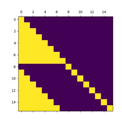
A visualization of the MonArc attention mask

This mask makes it such that attention for each $\hat{x_{t}}$ is computed as if it were the last token in the sequence $[x_{< t}, \hat{x_{t}}]$ . Note that this also requires that the position id passed for $\hat{x_{t}}$ is $t$ , not $t + T$ . Recounting our architectural design above, this is exactly the format for computing the energy of $\hat{x_{t}}$ .

Finally, we use the hidden states of $x$ to compute the cross-entropy loss of $p_{L} M$ and the positive sample portion of the RLM gradient, while the hidden states of $\hat{x}$ are used to calculate the negative portion of the RLM gradient.

In all, each training step requires one forward pass of $T$ tokens and one forward and backwards over $2 T$ tokens. In practice, training takes about 2.3 times longer than for a standard LLM for short sequences. For long sequences, the double-length attention dominates with its O(T^2) complexity, and MonArc training takes up to 4 times longer.

Experiments

We test our method using a standard Llama backbone, with pre-block layernorms and rope embeddings on each attention head. Our dataset is the CC-MAIN-2024-18 subset of fineweb, tokenized using the GPT-2 tokenizer. We use a context length of 512, with shorter sequences packed together.

Our 163M model configuration uses the same hyperparameters as GPT-3 Small, and our 430M model uses those of GPT-3 Medium. Further config information can be found in the config files. In each experiment, the energy head was initialized with zeros.

Results

First, we look at the loss curve of our small configuration over 50 billion tokens training from scratch. In the graph below, Baseline-LM represents the NLL of a standard LLM, MonArc-LM represents the NLL of the $p_{L M}$ component of the MonArc model, and MonArc-ELM represents the estimated NLL of the composite MonArc model.

To estimate the composite MonArc NLL, we assume that Z=1 as the regularizing component of the RLM loss function promotes. Closer inspection using the bounds found in section 3.2 of this previous work showed that this is a good approximation the true NLL.

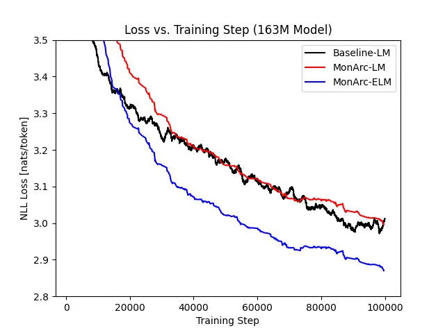
Graph of the 163M Model training loss

We see that that MonArc is about twice as data efficient as a standard LLM. Accounting for MonArc using more compute per step, this means that MonArc has about the same training compute efficiency as a standard LLM.

Second, we trained a standard LLM using our 430M configuration from scratch for 50 billion tokens. Then, we perform continued pretraining on that model for another 10 billion tokens, this time adding a MonArc head. For comparison, we also continue training the standard LM for 10 billion tokens.

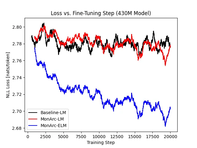
Graph of the 430M Model training loss

We see that the standard LM improves very slowly with continued training, while the MonArc model shows clear progress. The MonArc LM component also maintains similar performance to the standard LLM.

Future Work

Further experiments are obviously needed to prove MonArc's effectiveness. In particular, MonArc should be compared against a baseline LLM on reasoning benchmarks like MMLU. We theorize that focusing on each potential answer one-at-a-time in order to rerank them could have an outsized impact on reasoning performance as a form of test-time scaling.

Ablations are also needed to support our design decisions. Most pressing among them would be a comparison between the NCE and RLM losses. I am admittedly doing this write-up long after I actually performed these experiments, and can't find the NCE results. For now, just trust me that NCE and RLM led to very similar outcomes. That said, we still prefer the RLM loss because it is cool.

MonArc pretraining could also have interesting implications for finetuning on downstream tasks. It has already been shown by ELECTRA (the inspiration for MonArc) that token-level EBMs can yield formidable downstream performance in the bidirectional regime. MonArc may be particularly well-suited for process reward modelling, since it has already been conditioned to judge and evaluate the previous token.

#project