pBit

14 Dec, 2024

TLDR

Non-differentiable parameterizations (low-bit quantization, sparsity) can be approached by modelling parameters as random variables.
The local reparameterization trick is a low-variance and differentiable way to train random parameters.
The pBit method leads to successful training of language models with ternary quantization and up to 87% sparsity.
Sparse ternary quantization yields (potentially interpretable) repeated structures and parameter allocation patterns.

Links

Original Report: Sparse Ternary Transformers @ Weights & Biases

Introduction

Modern transformer language models can have 100s of billions of parameters. This makes them prohibitively memory and compute expensive, and unfeasible for the average consumer to run locally. To overcome this, methods have been introduced that lower the precision of weights from the usual 16 bits to 1.58 bits ("ternary networks" with weights in {+1, 0, -1}), or even 1 bit ("binary networks/BitNets" with weights in {+1, -1}). However, training these networks usually relies on a straight-through estimators (STE), which can be unstable and make distillation from existing networks difficult. This work replaces STEs with variational methods, which to the author's knowledge have not been scaled up to modern deep learning architectures.

Another way to reduce the cost of models is with "sparsity" - setting many weights to zero, so that they do not need to be explicitly stored or used in computation. For large models this is usually done with heuristic methods (such as setting weights with small magnitude to zero). However, those heuristics are often done independently of the gradient descent procedure, so optimal sparsity is unlikely to be achieved. Variational methods can help here too, since they combine gradient descent and sparsity in a unified framework.

We show that with some engineering, variational quantization and sparsity can be effective for modern transformers. We will also look at some interesting structures that arise from these methods and gain insights into how weights should be distributed in a transformer. We will also touch on explainability and describe how our method could be used to efficiently distill exisiting models.

Why use quantization and sparsity together, rather than exploring them separately?

As seen in the method section, variational sparsity is an easy extension of variational ternary networks. We have also found informally that training quantized sparse networks is easier than continuous sparse networks. In the later sections, we will also see how discrete weight values in addition to sparseness having allows us to make some interesting insights into the network's structure.

Variational dropout to create sparsity in full-precision weights for image classification: arxiv.org/abs/1701.05369
The local reparameterization trick: arxiv.org/abs/1506.02557
Binary weight transformers: arxiv.org/abs/2310.11453
Ternary weight transformers: arxiv.org/abs/2402.17764 and arxiv.org/abs/2504.12285
Distilling extremely quantized networks: huggingface.co/blog/1_58_llm_extreme_quantization

Methods

We represent every weight in the transformer's matrices with a probability distribution, rather than a fixed value. After training, we sample from that distribution to get our final weights. We want our expected loss after this sample to be as low as possible. This gives us the following training objective (see related works for more rigorous treatment):

θ^{'} = {argmin}_{θ} 𝔼_{\hat{θ} ~ θ} [ℒ (\hat{θ})]

Variational BitNets (VBNs)

To start with, consider the simple case of a variational BitNet (VBN):

w \in {+ 1, - 1} ~ 2 Bern (p) - 1

Here, weights are +1 with probability $p$ , and -1 otherwise. Training $w$ directly would be difficult, because it is discrete, and we can't perform backpropagation into $p$ . However, we can get around this using the local reparameterization trick.

Consider the linear operation $y = W x$ with $y \in ℝ^{m}$ , $x \in ℝ^{n}$ , and $W$ is an m by n matrix of stochastic weights as described above. We will use $P$ to represent the matrix of probabilities that parameterize $W$ . The j-th value of $y$ is computed as $y_{j} = \sum_{i = 1}^{n} w_{j, i} x_{i}$ . This makes it a sum of many random variables, so we can approximate it using the central limit theorem.

The central limit theorem states that the sum of many random variables will approach a gaussian distribution with mean $μ = \sum μ_{i}$ and variance $σ^{2} = \sum σ_{i}^{2}$ . When applied to the case above, we have $μ (w_{j, i} x_{i}) = (2 p_{j, i} - 1) x_{i}$ and $σ^{2} (w_{j, i} x_{i}) = 4 p (1 - p) x^{2}$ . The entire linear operation then becomes:

y = W x ~ 𝒩 (μ (x), σ^{2} (x))

μ (x) = 2 P x - 1_{m, n}

σ^{2} (x) = 4 (P ⊙ (1_{m, n} - P)) (x^{⊙ 2})

This can be efficiently computed with 2 matrices multiplications, and a few elementwise operations. More importantly, it means that we can use the well-known reparameterization trick to for optimization:

\nabla 𝔼_{y} [ℒ (y)] = \nabla 𝔼_{ϵ ~ 𝒩 (0, 1)} [ℒ (μ (x) + σ (x) ϵ)]

Variational Ternary Networks (VTNs)

Networks with "1.58 bit" weights in {+1, 0, -1} have been shown to outperform BitNets, and also allow us to use sparsity. To represent the weight of a variational ternary network (VTN), we use two Bernoulli variables subtracted from one another:

w \in {+ 1, 0, - 1} ~ B e r n (p_{+}) - B e r n (p_{-})

μ (w) = p_{+} - p_{-}

σ^{2} (w) = p_{+} (1 - p_{+}) + p_{-} (1 - p_{-})

We can then optimize our weights by extending the method we described for VBNs. However, we have found that directly optimizing $p_{+}$ and $p_{-}$ does not work very well, often ending up in a degenerate high-variance state of $p_{+} \approx p_{-}$ . In order to make our loss as low as possible, we want to maximize the signal to noise ratio in the network, which means having as low of variance as possible for a given mean. To do this, we can directly calculate the lowest variance $p_{+}$ and $p_{-}$ for a given $μ (w)$ :

p_{+}^{'} = {\begin{matrix} μ (w) & if μ (w) \geq 0 \\ 0 & else \end{matrix}

p_{-}^{'} = {\begin{matrix} 0 & if μ (w) \geq 0 \\ μ (w) & else \end{matrix}

So in practice, we optimize a single variable $μ (w)$ , with $μ (W)$ representing an entire matrix of $μ (w_{j, i})$ , which can be converted into implicit probabilities $p_{+}^{'}$ and $p_{-}^{'}$ when we need them. Putting it all together, we can efficiently calculate $y = W x$ as a gaussian distribution like we did before:

y = W x ~ 𝒩 (μ (x), σ^{2} (x))

μ (x) = μ (W) x

σ^{2} (x) = (| μ (W) | ⊙ (1 - | μ (W) |)) (x^{⊙ 2})

Since $y$ is again a normal distribution, we can then apply the reparameterization trick as we did for BVNs.

Sparsity

To enforce sparsity, we want to have as many expected zeros in our sampled weights as possible:

ℒ_{s p a r s e} (θ) = 𝔼_{\hat{θ} ~ θ} [\sum_{k} (\hat{θ} \neq 0)]

With the ternary representation from the previous section, the sparsity loss can be calculated as follows (where $ℳ$ is the entire neural network):

ℒ_{s p a r s e} (ℳ) = \frac{\sum_{W \in ℳ} \sum_{j = 1}^{m} \sum_{i = 1}^{n} | μ (W_{j, i}^{(k)}) |}{numel (W)}

The full loss then becomes the following, with $λ_{sparse}$ as a hyperparameter referred to as the "sparsity penalty":

L_{t o t a l} (θ) = ℒ (θ) + λ_{sparse} ℒ_{sparse} (θ)

Our framework is also able to handle more complicated sparsity penalties, such as encouraging structured sparsity for better hardware compatibility, but we leave it for future work.

Engineering

We describe some engineering tricks that we have found to vastly improve the effectiveness of our method.

The first trick is the representation of $μ (w)$ which needs to stay in the range [-1, 1]. The most obvious way to enforce this is by parameterizing it as $μ (w) = sigmoid (u)$ and optimizing $u$ with SGD. However, found two problems with this idea:

$σ^{2} (w)$ can only reach zero at $μ (w) = \pm 1$ , which would require $u$ to go to $\pm inf$
$u$ often takes on very high or low values early in training, which are difficult to recover from later. We found a better parameterization in the form of $μ (w) = clip (u, - 1, 1)$ , clipping $u$ to the range [-1.05, 1.05] after each gradient step. The linear relationship between $u$ and $μ (w)$ makes training dynamics similar to a regular network, and the clipping keeps values in the desired range.

We clip u to [-1.05, 1.05] instead of [-1.0, 1.0] to give it some room where it can sit with exactly zero variance, otherwise it will "bounce off the walls" of its range and have trouble achieving zero variance.

The second trick is the scaling of $u$ . For a linear layer with $n$ inputs, weights typically have a magnitude on the order of $1 / \sqrt{n}$ . The form above has $u$ with a magnitude on the order of 1, which would require us to adjust our learning rate. To fix this, we set $μ (w) = c l i p (u \sqrt{n}, - 1, 1)$ and clip $u$ to $[- 1.05 / \sqrt{n}, 1.05 / \sqrt{n}]$ after each gradient step. This simple adjustment allows us to use the same learning rates as in standard training.

The third "trick" (this one's less of a trick and more of a note) is to initialize $u ~ Uniform (- 1 / \sqrt{n}, 1 / \sqrt{n})$ and scale the output of the linear layer by 2 to keep unit variance on the outputs (similar to Kaiming initialization).

The fourth trick is to apply an elementwise scale and bias to both the inputs and outputs of every linear layer. The scaling helps recover some of the expressiveness lost by quantization, the input bias helps reduce the variance of the linear layer's outputs, and the output bias corrects adjustments made by the input bias. For layers preceded by a layernorm (ex. QKV), we already have input scaling and bias, and don't need to add them redundantly.

I might later write an appendix on why input bias reduces variance, but for now I leave that as an exercise for the reader. My succinct note is that it is analogous to the expected value estimate often used to reduce the variance of the REINFORCE algorithm.

The fifth trick is applying a linear warmup to the sparsity penalty. This prevents the networks from collapsing to mostly zeros or other undesirable states early in training.

The final trick is applying a linear warmup to the gaussian noise in the reparameterization trick. This can be described by letting $y = μ (x) + σ (x) ϵ, ϵ ~ 𝒩 (0, α^{2})$ , with $α$ linearly increasing from 0 to 1 throughout training (increasing it above 1 could be another interesting experiment). To see why this helps, consider the plot of $μ$ versus $σ^{2}$ as described in the Variational Ternary Networks section. We see that low variance can be achieved near -1, 0, and 1. These areas become local minima for the loss function and cause the model to get stuck in suboptimal states. Warming up the noise scale applies an annealing-like effect that allows $μ$ to travel more easily during early training, and lets the model find better minima.

Experiments

We test our method on the language modeling task with a standard decoder-only transformer architecture, with pre-block layernorms and rope embeddings on each attention head. Our dataset is the CC-MAIN-2024-18 subset of fineweb, tokenized using the GPT-2 tokenizer. We use a context length of 512, with shorter sequences packed together.

We use the same model configuration and hyperparameters as GPT-3 Small. Further config information can be found in the project and model checkpoints.

The learning rate decayed to 1/10 of its starting value after 20,000 steps and stayed at that point and stayed there for the rest of training.

The "mini-control" run used standard mixed precision with no sparsity, "mini-ternary-dense" was a variational ternary network with no sparsity penalty, and "mini-ternary-sparse" has a sparsity penalty of 5.

The noise and sparsity penalty both linearly warmed up to their final value over 15,000 steps.

Results

pbit_plots

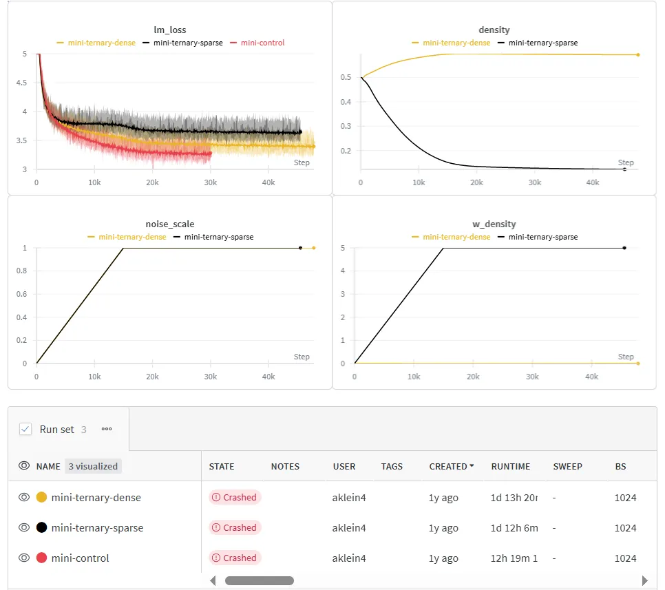
We see that the dense variational ternary network performs slightly worse than the control, and the sparse one performs slightly worse than that. However, these results are encouraging considering that these models are small, and both quantization and sparsity have been shown to degrade performance more in smaller networks.

If should also be emphasized that with a sparsity of ~87%, mini-ternary-sparse ends up with just ~16,000,000 non-zero non-input-embedding parameters. This makes it almost 3 times smaller than any other transformer-based general language models that the author can find (Pythia 70M has ~45,000,00 non-input-embedding parameters). The fact that it still converges to a reasonable loss is remarkable in itself.

Pythia 70M is described by its authors as having "18,915,328 non-embedding parameters". However, this does not count the language modelling head, which has more than 25,000,000 parameters (and is not tied to the input embeddings). This makes the use of "non-embedding parameters" a bad comparison with our experiments, since we also reduce the size of the head.

We therefore use the term "non-input-embedding parameters" to describe all parameters that are not in the input embeddings (all transformer blocks, normalizations, and the language modelling head). This is a useful measurement because it describes parameters that are used every forward pass, unlike input embeddings which are only fetched for their corresponding token.

Analysis

Cross-Matrix Correlations

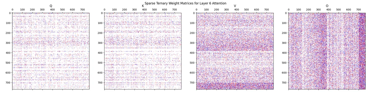
We find that in cases where the weight matrices have structure (such as the QKV and O attention matrices being broken into separate heads), we find that the sparsity follows that structure. For example, in the image below, we see that denser V matrix heads correspond to denser O matrix heads. We also see that denser Q matrix rows correspond to denser K matrix rows.

Below, we see a visualization of the QKVO attention matrices from the mini-ternary-sparse run. Blue = +1, White = 0, Red = -1.

pbit_weights

Parameter Distributions

We can look at the sparsity levels of each matrix in the model to see how the optimization process distributed the location of weights. Below are the parameter density levels for different matrices across layers for the mini-ternary-sparse run.

pbit_densities

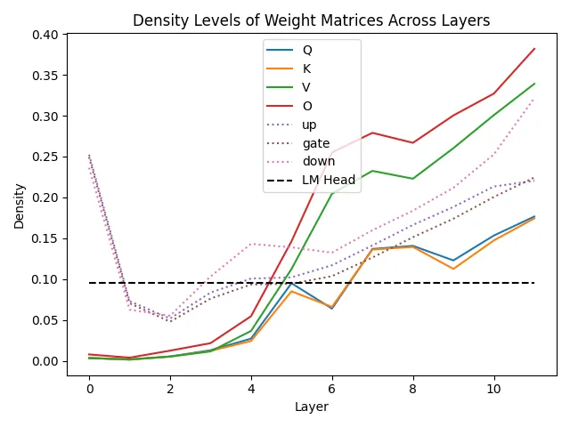
We see significant correlation between weight matrices that work together (Q and K, V and O, the MLP matrices). We also see that early layers have very few parameters and later layers have more, with the exception of the first two MLPs.

This analysis could be valuable for the design of dense transformers, to help engineers decide how to distribute the parameters and compute of a model. For example, our findings match those of OpenELM, who showed that using larger MLPs in later layers is more efficient.

Repeated Structure

The sparsity patterns of the matrices (visualized above) show remarkable structures that could be of interest for interpretability and knowledge representation research. For example, there exist non-trivial (with many- non-zero elements) matrix rows that are exactly the same across layers. This means that for some rows in the 3rd Q matrix, there exist rows in the 4th and 5th Q matrices that are exactly the same! We intend to do further research on this subject to determine the semantic importance of these rows, and whether they correspond to interpretable features.

Future Work

Distillation

While ternary networks have shown promise when pretrained, researchers have found it difficult to distill them from existing standard networks. To this end, we believe that our method could make distillation easier. To see why, consider an existing model with a weight matrix $W \in ℝ^{n, m}$ . To convert it to a variational ternary network, we set $u_{j, i} = \frac{W_{j, i}}{\sqrt{n} max (| W |)}$ and fill the output scale vector with $max (| W |)$ ((a similar conversion can be achieved for a variational BitNet). Then, when the noise scale is zero, the ternary network will exactly recover the existing network.

Scaling by the maximum magnitude of the entire matrix is the simplest way to do it. We could also scale by the row and/or column maximums, setting input and output scales appropriately. The maximum may also be an outlier, so scaling by something like 3 standard deviations of the weight values might be better (clipping values that fall outside of U's range). However, this would be at the cost of perfectly recovering the existing network.

As the noise scale increases throughout training, the weights will be able to smoothly transition into quantized values while maintaining a low loss throughout. This is in contrast to straight-through estimator (STE) based distillation, which mangles the network at the start of training and attempts to recover performance by the end. STE methods also lack an obvious conversion between existing weights and quantized form, relying on heuristics.

Pruning

When fine-tuning a general-purpose language model to a specific task, it's possible that not all of its weights will be needed for that task. Distillation with a sparsity penalty could be a way to easily reduce the parameter count of models during fine-tuning, with the advantages described in the Distillation section above.

#project