ZEBRA (WIP)
TLDR
- Latent reasoning can be framed as a hierarchical VAE where each token is a latent level.
- Using an IAF encoder, we can train these models entirely in parallel while maintaining serial inference and its benefits.
- New regularization techniques make it possible to scale HVAEs to unprecedented depth (384 levels) without posterior collapse.
- Outperforms a matched 1.7B LLM baseline by an average 2.1% on reasoning benchmarks after only 4B tokens of adaptation.
Links
Code: aklein4/zlm @ github (warning: not prepared for other human eyes, yet)
Model Weights: aklein4/zebra-1.7b-preview @ huggingface
Introduction
Chain-of-thought (COT) reasoning models that “think before they speak”, such as OpenAI o1 and DeepSeek R1, have significantly advanced the frontier of language model performance. However, this paradigm faces two key limitations:
- At the end of each forward pass through the model, all information is disregarded except for a single discrete token. This token can contain at most (approximately 18) bits of entropy, far less than what's contained in the model's rich hidden state.
- Textual COT reasoning relies on the built-in language capabilities of LLMs. Modality-specialized models for science (such as AlphaFold and ProGen) lack natural reasoning mediums, and therefore cannot benefit from COT reasoning.
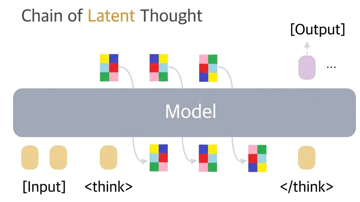
In this work, we introduce ZEBRA (Z-spacE Based Reasoning Architecture), a new type of generative model that reasons in continual space. ZEBRA addresses both of the limitations above:
- At the end of each forward pass, ZEBRA saves its hidden state to a continuous high dimensional vector, which has a much higher information capacity than a discrete token. This alleviates the information bottleneck of textual COT.
- Rather than bootstrapping human language, ZEBRA develops its reasoning patterns from scratch through end-to-end optimization. This makes it applicable to any domain.
Related Work
COCONUT introduced the concept of latent COT reasoning with continuous vectors. However, COCONUT (and the many similar methods that have followed) still face significant obstacles:
- At training time, latent vectors are computed serially across the reasoning chain, and backpropagation is performed serially through time. This makes training much slower than the typically parallel training of transformers.
- No stochastic sampling is performed until the output stage, so there is no reduction in entropy during reasoning. This means that possible responses are not narrowed down until the end, and the model must reason across every possible response without focus.
Other lines of work use reinforcement learning for training, which is notoriously sample-inefficient and usually still requires serial policy rollouts.
As we will see, ZEBRA does not suffer from any of these issues.
Methods
At its core, ZEBRA is a Hierarchical Variational Autoencoder (HVAE). As a matter of fact, ZEBRA is the deepest HVAE ever constructed. It is an order of magnitude deeper than the previous deepest.
Formulation
The generative modelling formulation of a ZEBRA model is the same as other conditional VAEs:
Since an N-depth ZEBRA model is specifically a conditional HVAE, it admits an autoregressive form of :
In its basic form, the ZEBRA model is trained using the same (beta) ELBO loss as standard VAEs. We will add some bells and whistles later to improve training dynamics.
Our posterior is also an N-depth autoregressive model:
Here and in our code, we will refer to the model that computes the posterior as the "encoder", the model that computes the prior as the "generator", and the model that computes the output as the "decoder".
We may also omit the condition (which can be thought of as the "prompt") for brevity.
Architecture
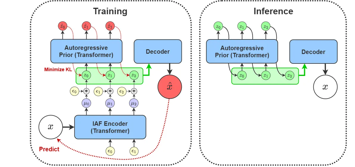
The key insight of ZEBRA is that we can take the usual HVAE architecture, where z is sampled depth-wise at each layer of the deep neural network, and turn it on its side. Instead of sampling at the i-th layer of the network, we always sample z from the last layer. Autoregression is performed on the sequence axis. We compute using a causally masked transformer where is embedded in the t-th token, just as an LLM computes . This allows us to grow N without growing the depth of our network, and it also allows us to calculate for all in a single forward pass.
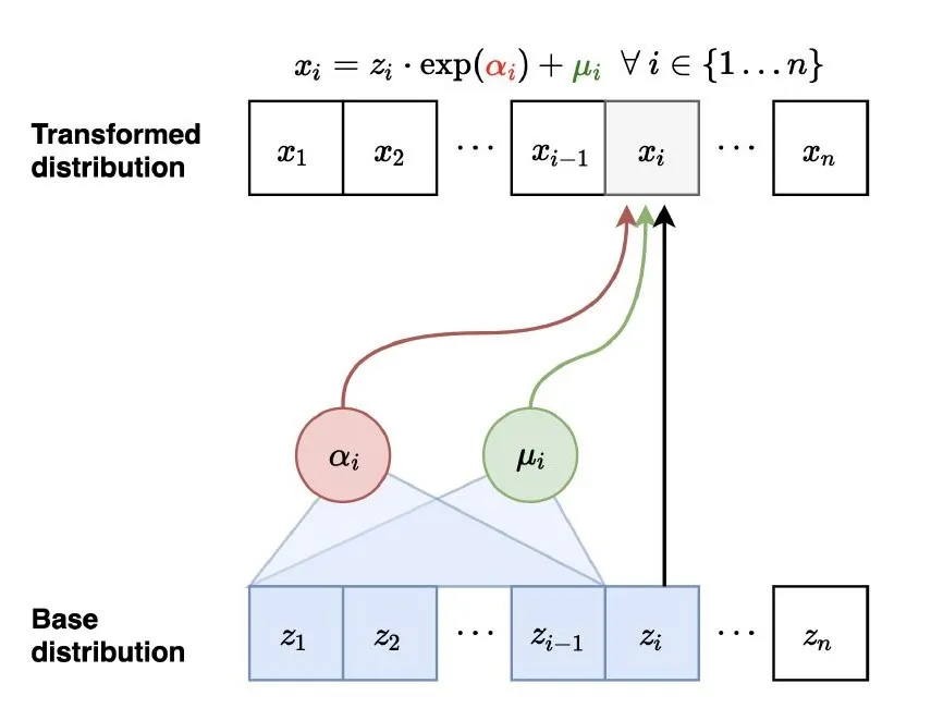
The sequence-wise formulation of ZEBRA also enables one of its most important properties: parallel training. By designing the encoder as an Inverse Autoregressive Flow (IAF) along the sequence dimension, we can draw samples from the posterior in a single forward pass. This is done using a causally masked transformer where is computed using the hidden states at position t, and the noise used to sample from (this will be elaborated on shortly) is passed into the transformer at position . This is shown in the IAF diagram below.
In our formulation, the encoder IAF is conditioned on both and . To realize this architecturally, we put the tokens corresponding to and at the start of the sequence, so that the IAF tokens can causally attend to them. Similarly, we put the tokens at the start of the input to generator/decoder transformer (we use a single transformer for both) and the tokens at the end. This allows the tokens to causally attend to and the output tokens to attend to both and .
Latent Parameterization
We parameterize our posterior distribution using an isotropic gaussian. We found that using a fixed diagonal variance significantly improves training stability over a dynamic one.
At training time, we can sample from this distribution using the reparameterization trick:
The noise here is the noise that is fed into the IAF model as mentioned previously.
For increased expressiveness, we parameterize our prior distribution using a diffusion head, which still admits calculation of an ELBO.
TODO: More explanation on the diffusion head
Training Process
Given our design, each training step goes as follows:
- , , and are fed into the encoder, yielding .
- is calculated using the reparameterization trick with , , and .
- , , and are fed into the generator/decoder model.
- The reconstruction loss is calculated by applying the cross-entropy loss to logits calculated from the hidden states. The hidden states of are used to calculate the logits predicting , just like in an LLM.
- The loss is calculated using the diffusion ELBO.
- Gradients from the losses are backpropagated into the generator/decoder, and further propagate into the encoder through using the reparameterization trick.
That's the jist. Breaking down each of the losses, we see that:
- is pushed towards making easy to predict.
- is pushed towards being easy for the generator to predict given .
- is pushed towards making it easier to predict .
These forces work to optimize the latent space into a reasoning medium, where reasoning tokens are both easy to generate and useful for future computation.
Posterior Collapse
A common pitfall of VAEs with expressive decoders is posterior collapse: the decoder can get low reconstruction loss without using at all, which means that the only pressure going to is the KL penalty. This causes the posterior distribution to degenerate into an uninformative state. We take the following measures to prevent this.
, the scale on the KL penalty, is zero until the reconstruction loss is below a set threshold. At that point, increases linearly across a number of warmup steps to . This induces a "hooking" behavior in the network: once the decoder has tasted the information in , it will not let it go as long as still carries information. As long as , will have a stronger incentive to be informative than to collapse, so it will continue to carry information.
Furthermore, gradients are not passed into the generator from the diffusion head until the hooking threshold is reached, after which point they are linearly warmup up to full scale. We found this to greatly increase early training stability, and prevent the model from chasing its own tail with inter-z dependencies.
TODO: explain how \beta is modulated to keep the reconstruction loss at a set value similar to delta-VAE
Hierarchical Collapse
Another common pitfall specific to HVAEs is that individual levels of will go unused and collapse. We use a simple hyperparameter-free method to prevent this.
At each step, the batch-wise mean of , denoted as is calculated at every . We then calculate the position-wise loss weights:
We then calculate the weighted KL penalty:
This method assigns low KL penalties to positions with lower average divergence, while keeping the total penalty constant.
We found best performance when only applying this scaling gradients of the encoder directly from the KL (the encoder still gets regular gradients through the generator).
Spectral Collapse
Another issue that we noticed was that a tiny fraction of the directions in the space of explained nearly all of the variance. To address this, we perform spectral batch normalization to . This is done by calculating the batch-wise covariance of separately for each , and multiplying each by to whiten them. Gradients are passed through the whitening process. While this cost may become prohibitive for large dimensionality, we found it doable for 32 and 64 dimensional latent vectors.
Noise Warmup
In some cases, especially when the decoder is a pretrained LLM, we encountered posterior collapse even when there was no KL penalty. We believe that this is because the high signal-to-noise ratio at the start of training prevents the decoder from ever making use of the latents. To fix this, we don't apply noise until the previously mentioned reconstruction loss threshold is passed. At that point, we linearly increase the standard deviation of the noise from 0 to its final value. After that, we proceed with the rest of the warmup phases as described in the Posterior Collapse section.
Experiments
Models
Our main experiments were performed using the pretrained HuggingFaceTB/SmolLM2-1.7B model. Both the encoder and the generator/decoder were initialized from this model.
TODO: explain initialization scheme in more depth
We used a maximum input length of 256 tokens, a latent depth of 384 tokens, and a maximum output length of 512 tokens. We set the number of dimensions in to be 32.
As a baseline, we continued pretraining a standard HuggingFaceTB/SmolLM2-1.7B model using the same hyperparameters and data. To maintain parity with the ZEBRA model, the cross-entropy loss for this model was only calculated on the output tokens of each sequence.
Data
Our training dataset was comprised of a mixed combination of web, code, chat, math, MCQA, and reasoning data. It can be found at pre-tokenized using the SmolLM2 tokenizer at aklein4/seq2seq-mixed-pretraining-SmolLM2.
TODO: go into more depth about the data
Notably, to make aide in later evaluation, we specifically formatted a fraction of the MCQA and math data to either have the answer at the very start or very end of the response, elicited by a corresponding prompt. This defined template makes answer extraction much easier.
Training
We trained our model for approximately 4 billion output tokens. This was performed over the course of several days on v4 TPUs through Google Cloud. Note that this means ZEBRA adaptation represents less than 0.1% of the model's total training tokens 1.
Results
Benchmarks
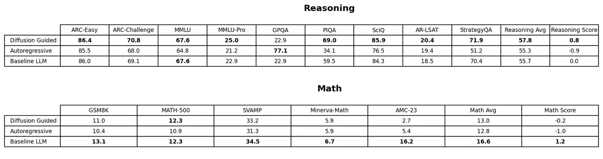
This table shows the results of various models on math and reasoning benchmarks. We have a ZEBRA model with a diffusion head (with classifier-free guidance), a ZEBRA model with an autoregressive head, and a standard LLM (no COT). All checkpoints have been continual pre-trained for 2B tokens on the same data and with the same settings as above.
The "Score" column represents the model's average z-score on each benchmark using that benchmark's corresponding mean and variance across models 2.
We see that the diffusion head ZEBRA model is the strongest on reasoning while the standard LLM leads on math. We also see a few standout scores for the ZERBA models: 77.1% on GPQA for the autoregressive head, and 69.0% on PIQA for the diffusion head.
Given the limited amount of adaptation training, we expect the performance of ZEBRA to become more favorable compared to the standard LLM as training continues, especially considering that the standard LLM didn't need to recover from destructive changes.
ELBO
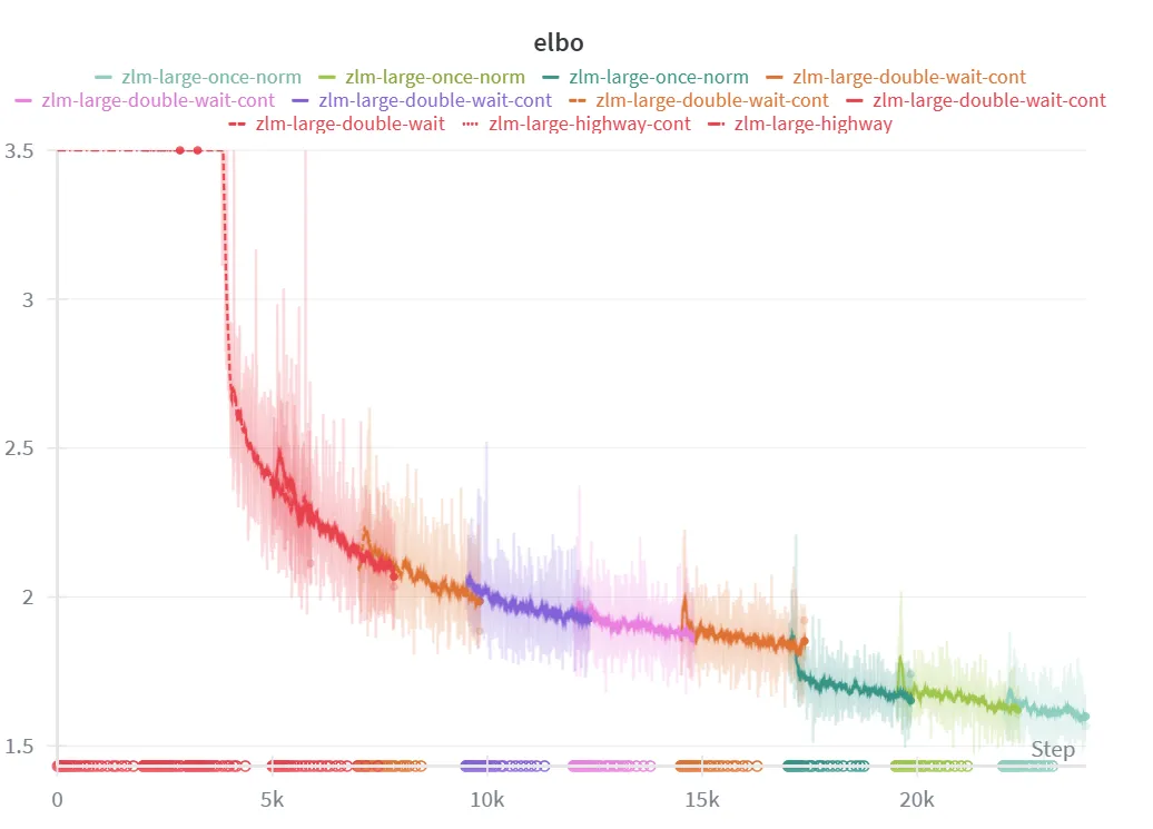
Above is a graph of the (negative) ELBO per token throughout training steps. We see that it consistently decreases throughout training and reaches about 1.6 by the end. For reference, a HuggingFaceTB/SmolLM2-360M model trained on our data reaches a cross-entropy of 1.5, and our baseline model reaches 1.15 in a similar number of steps. We believe that the difference between ZEBRA and the LLMs will continue to close with further training, given that our model has only been adapting to the ZEBRA objective for 4B tokens (compared to the trillions of tokens used to train SmolLM2 using a standard LLM objective). A portion of the difference could also be due to the gap between the ELBO and the true log likelihood, which we expect to be nontrivial due to the complexity of our distributions.
The multiple colors on the graph correspond to training restarts due to TPU device failure and other issues. The sudden downward jump at around 17K steps is due to the disabling of spectral batch normalization, which allowed the model to slightly collapse to a lower loss but less interesting state.
Reconstruction Loss
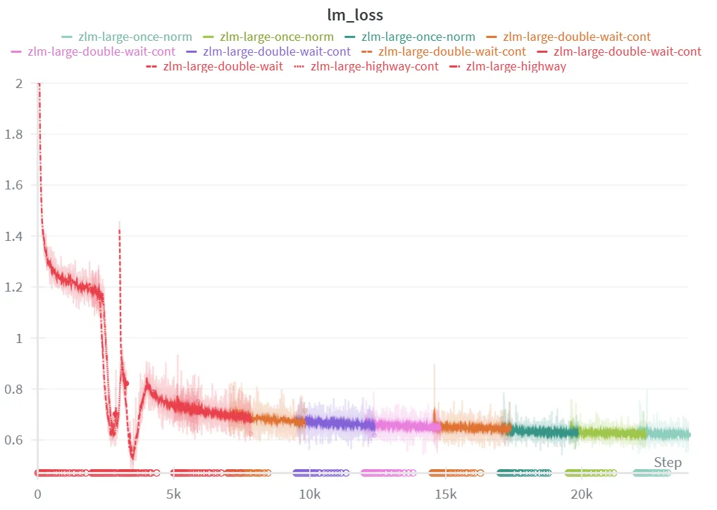
Above is a graph of the reconstruction loss (cross-entropy on the output tokens) throughout training. We see that characteristic hooking behavior at around 3,000 steps, after which the KL penalty kicks in causing the reconstruction loss to rise and fall again once the KL penalty evens out.
Hierarchical Collapse
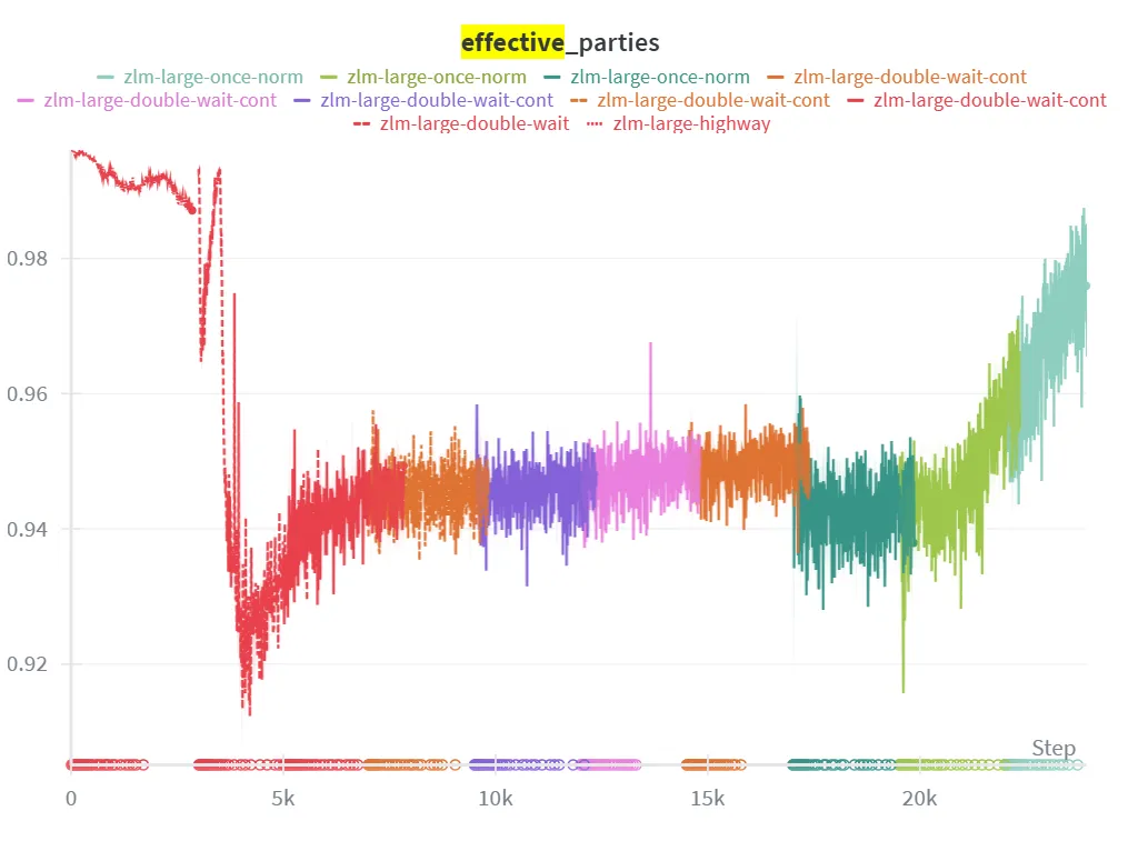
To measure the proportion of latent positions that have not collapsed, we adopt the effective number of parties metric from political science. Recounting from the KL weighting section, we define the proportion of effective parties as:
This metric is easily interpretable. If then all positions have equal average KL, if then the KL is concentrated in half of the positions, if then the KL is concentrated in a third, and so on.
We find that our KL weighting method is effective at distributing the KL evenly across positions, with reaching no lower than 0.9 throughout training.
Spectral Collapse
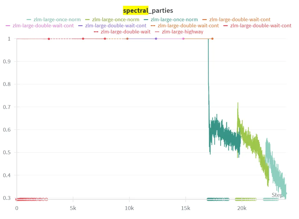
In the graph above, we apply the effective parties metric to the principle components of . Here, we calculate the effective parties over the explained variance of each batch-wise principle component. This is done separately for each position, and averaged across positions to get a final value.
We see that for the first ~17,000 steps, all principle components contribute equal amounts of explained variance. This is the direct result of our spectral normalization. Once we remove spectral normalization around step 17,000 we see the explained variance quickly consolidate into about 30% of the principle component directions. Since our latents had 32 dimensions, this means that only about 10 of them were being used.
Example Generations
Below are 3 example responses from our ZEBRA model. For each generation, we use DDIM sampling in the diffusion head and greedy (deterministic) sampling on the output token logits. To show that the output depends on , we provide two responses for each input with the only difference being the noise seed at start of the DDIM sampling chains.
The first example shows the ZERBA model correctly answering a multiple choice reasoning question (the correct answer is B).
 === INPUT ===
<|im_start|>system
Place the final answer to the following question inside of a \boxed{} command. This must appear at the start of your response before any other text.<|im_end|>
<|im_start|>user
One year, the oak trees in a park began producing more acorns than usual. The next year, the population of chipmunks in the park also increased. Which best explains why there were more chipmunks the next year?
A: Shady areas increased.
B: Food sources increased.
C: Oxygen levels increased.
D: Available water increased.<|im_end|>
<|im_start|>assistant


 === OUTPUT 1 ===
\boxed{B}
The oak trees producing more acorns the next year implies an increase in the quantity of acorns, which likely stimulated the chipmunk population. While food availability is often the dominant factor in wildlife ecology, the specific choice of "food sources" (B) is the most fitting explanation.

The oak trees' excessive acorn production could have been a result of climate conditions, altered soil composition, or other natural factors, pushing the tree population to outcompete local vegetation, leaving more acorns for the chipmunks. This aligns with the observed increase in chipmunk numbers.

Other options are less likely:
- **A (Shady areas)** could correlate with wildflower/nut production, but the question does not mention vegetation changes.
- **C (Oxygen levels)** is unlikely, as air quality is unlikely to influence acorn production.
- **D (Water)** is not relevant given the geographic context of the oak trees (water sources tend to be restricted, particularly in places like the African savanna where the oak trees are native).

The most plausible explanation is the increased availability of acorns due to the higher acorn production, making **B** the best answer.

\boxed{B}<|im_end|>

 === OUTPUT 2 ===
\boxed{B}
The increased chipmunk population in the park the next year is best explained by the **food source increase**. This is because acorns are the chipmunks' primary food source, and when the oak trees produced more acorns the previous year, the availability of this food source substantially expanded. While the original explanation (A) of shyer areas is plausible, it relates to the cause of oak tree production, not the observed survival of chipmunks. The most direct and plausible answer is that the increased food supply (B) provided increased sustenance after the survival of the chipmunks.

Other options are less likely:
- **C (Oxygen levels)**: Oxygen is required for photosynthesis, but this does not directly explain the food source increase due to acorns.
- **D (Water)**: Water is not the primary food source for chipmunks, and higher water levels (e.g., due to rainfall or weather) would not influence the oak tree productivity.
- **A (Shady areas)**: While shady areas can support oak trees, the question does not specify this as a known cause of the higher oak crop.

The answer is **B** because the food source increase after the favorable acorn conditions directly accounts for the increased chipmunk population.

\boxed{B}<|im_end|>
The next example shows the ZEBRA model correctly answering a grade school math question (the correct answer is 108).
 === INPUT ===
<|im_start|>user
Bob had a farm with animals. He had 12 cows and twice as many sheep. He decided to buy 3 pigs for every sheep he had. How many animals were on the farm after the transaction?<|im_end|>
<|im_start|>assistant


 === OUTPUT 1 ===
Let's compute the number of animals after the transaction.
Bob had 12 cows, which is 12 * 1 = 12.
He also had twice as many sheep, so he had 12 * 2 = 24 sheep.
Now he needs to add 3 pigs for every sheep he has. So he needs 24 * 3 = 72 pigs.
The total number of animals is thus 12 + 24 + 72 = 36 + 72 = 108.
Thus Bob had \boxed{108} animals on the farm after the transaction.<|im_end|>

 === OUTPUT 2 ===
To determine the total number of animals on Bob's farm after the transaction, we need to follow these steps:

1. Calculate the number of sheep Bob had.
2. Determine the total number of pigs Bob had.
3. Add the number of cows, sheep, and pigs.

First, Bob had 12 cows. He decided to buy 3 pigs for every sheep he had. Since he had twice as many sheep as cows, the number of sheep is:
\[
\text{Number of sheep} = 2 \times 12 = 24
\]
\[
\text{Number of pigs} = 3 \times 24 = 72
\]

Next, we add the number of cows, sheep, and pigs:
\[
\text{Total number of animals} = 12 + 24 + 72 = 108
\]

To confirm, we can also express this as:
\[
\text{Number of cows} + \text{Number of sheep} + \text{Number of pigs} = 12 + 24 + 72 = 108
\]

Therefore, the total number of animals on the farm after the transaction is \(\boxed{108}\).<|im_end|>
The final example shows the ZEBRA model failing on a more difficult math question (the correct answer is 27).
 === INPUT ===
<|im_start|>system
Place the final answer to the following question inside of a \boxed{} command. This must come at the end of your response, and no other text should come after it.<|im_end|>
<|im_start|>user
What is the smallest positive perfect cube that can be written as the sum of three consecutive integers?<|im_end|>
<|im_start|>assistant


 === OUTPUT 1 ===
We know that the sum of three consecutive integers is odd, so one of the integers is odd and the other two are even.

The smallest perfect cube is $8^3 = 512$.

Now, we need to check the sum of three consecutive integers:
- Numbers 1, 2, 3: 1 + 2 + 3 = 6, odd.
- Numbers 2, 3, 4: 2 + 3 + 4 = 9, odd.
- Numbers 3, 4, 5: 3 + 4 + 5 = 12, even.

The smallest four consecutive integers whose sum is odd are 1, 2, 3, 4, producing sum 10, which is not perfect.

The smallest six consecutive integers whose sum is odd is 1, 2, 3, 4, 5, 6, producing sum 21, which is not perfect.

The smallest seven consecutive integers whose sum is odd is 1, 2, 3, 4, 5, 6, 7, producing sum 28, which is not perfect.

The smallest eight consecutive integers whose sum is odd is 1, 2, 3, 4, 5, 6, 7, 8, producing sum 36, which is not perfect.

So, the answer is $\boxed{8}$.
Final answer: \boxed{8}<|im_end|>

 === OUTPUT 2 ===
To find the smallest positive perfect cube that can be written as the sum of three consecutive integers, we use the formula for the sum of an arithmetic series.

Let:
- $x$ be the smallest positive perfect cube.
- $n$ be the number of terms in the series.
- $a$ be the first term of the series.
- $l$ be the last term of the series.

The formula for the sum of an arithmetic series is:
\[ S = \frac{n}{2} (a + l) \]

We want $x$ to be the sum of three consecutive integers, so:
\[ x = a + (a + 1) + (a + 2) = 3a + 3 \]

Equating this with the sum of the series:
\[ 3a + 3 = \frac{n}{2} (a + l) \]

Simplifying:
\[ 3(a + 1) = \frac{n}{2} (a + l) \]

Since $a$ is the first term, the sum of the series is $3a + 3$. We can solve for $n$ and $l$:
\[ 3(a + 1) = \frac{n}{2} (a + l) \Rightarrow 6a + 6 = \frac{n}{2} (a + l) \Rightarrow 12a + 12 = na + \frac{n}{2} l \Rightarrow 12a + 12 = \frac{n}{2} (a + l) \]

Comparing coefficients of $a$:
\[ 12 = \frac{n}{2} \Rightarrow n = 24 \]

Comparing coefficients of $l$:
\[ 12 = \frac{1}{2} \Rightarrow l = 24 \]

Thus, the smallest positive perfect cube is $x = 24^3 = 13824$.

The answer is:
\[ \boxed{13824} \]
Final answer: \boxed{13824}<|im_end|>
Future Work
Significant work remains to prove the effectiveness of the ZEBRA architecture. This includes:
- More thorough evaluation and benchmarks
- Ablations on key design decisions
- Scaling with larger models and more training
- Applying ZEBRA to other modalities (such as protein sequence generation)
- Reinforcement learning to incentivize mode-seeking reasoning.
Acknowledgements
Research supported with Cloud TPUs from Google's TPU Research Cloud (TRC).
Footnotes
SmolLM2-1.7B was trained on 11 trillion tokens.↩
I believe that this is a much more informative and honest way to aggregate performance than a simple mean over benchmarks when each occupies a different range.↩